How to Optimize Multidimensional Numpy Array Operations with Numexpr

This is a relatively brief article. In it, I will use a real-world scenario as an example to explain how to use Numexpr expressions in multidimensional Numpy arrays to achieve substantial performance improvements.

There aren't many articles explaining how to use Numexpr in multidimensional Numpy arrays and how to use Numexpr expressions, so I hope this one will help you.

Introduction

Recently, while reviewing some of my old work, I stumbled upon this piece of code:

def predict(X, w, b):
    z = np.dot(X, w)
    y_hat = sigmoid(z)
    y_pred = np.zeros((y_hat.shape[0], 1))

    for i in range(y_hat.shape[0]):
        if y_hat[i, 0] < 0.5:
            y_pred[i, 0] = 0
        else:
            y_pred[i, 0] = 1
    return y_pred

This code transforms prediction results from probabilities to classification results of 0 or 1 in the logistic regression model of machine learning.

But heavens, who would use a for loop to iterate over Numpy ndarray?

You can foresee that when the data reaches a certain amount, it will not only occupy a lot of memory, but the performance will also be inferior.

That's right, the person who wrote this code was me when I was younger.

With a sense of responsibility, I plan to rewrite this code with the Numexpr library today.

Along the way, I will show you how to use Numexpr and Numexpr's where expression in multidimensional Numpy arrays to achieve significant performance improvements.

Code Implementation

If you are not familiar with the basic usage of Numexpr, you can refer to this article:

Exploring Numexpr: A Powerful Engine Behind Pandas

Enhancing your data analysis performance with Python’s Numexpr and Pandas’ eval/query functions

Data Leads FuturePeng Qian

This article uses a real-world example to demonstrate the specific usage of Numexpr's API and expressions in Numpy and Pandas.

where(bool, number1, number2): number - number1 if the bool condition is true, number2 otherwise.

The above is the usage of the where expression in Numpy.

When dealing with matrix data, you may used to using Pandas DataFrame. But since the eval method of Pandas does not support the where expression, you can only choose to use Numexpr in multidimensional Numpy ndarray.

Don't worry, I'll explain it to you right away.

Before starting, we need to import the necessary packages and implement a generate_ndarray method to generate a specific size ndarray for testing:

from typing import Callable
import time

import numpy as np
import numexpr as ne
import matplotlib.pyplot as plt

rng = np.random.default_rng(seed=4000)

def generate_ndarray(rows: int) -> np.ndarray:
    result_array = rng.random((rows, 1))
    return result_array

First, we generate a matrix of 200 rows to see if it is the test data we want:

In:  arr = generate_ndarray(200)
     print(f"The dimension of this array: {arr.ndim}")
     print(f"The shape of this array: {arr.shape}")


Out: The dimension of this array: 2
     The shape of this array: (200, 1)

To be close to the actual situation of the logistic regression model, we generate an ndarray of the shape (200, 1)an. Of course, you can also test other shapes of ndarray according to your needs.

Then, we start writing the specific use of Numexpr in the numexpr_to_binary method:

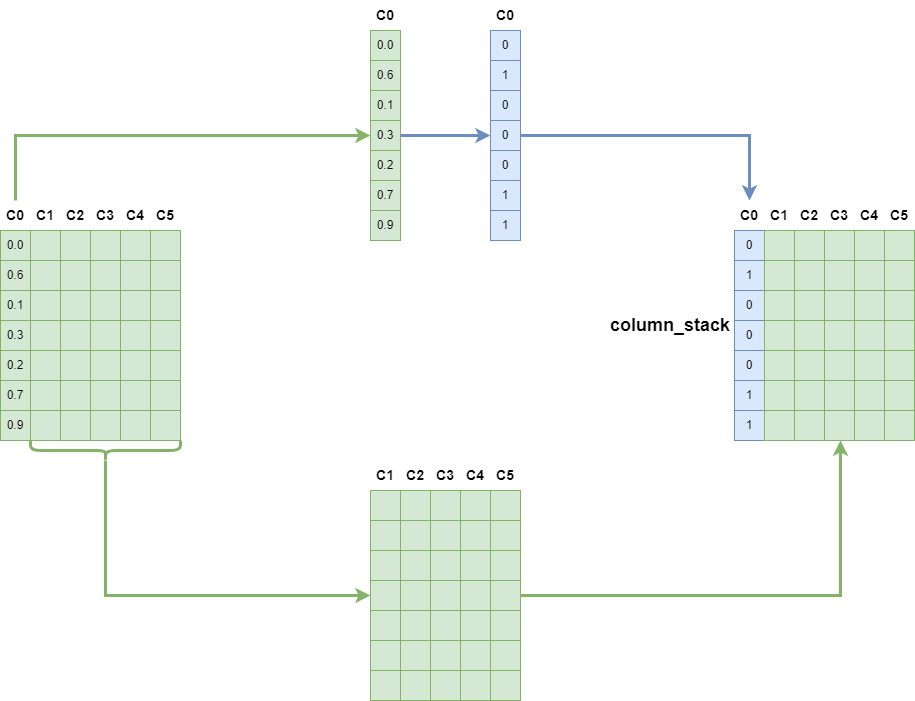
• First, we use the index to separate the columns that need to be processed.
• Then, use the where expression of Numexpr to process the values.
• Finally, merge the processed columns with other columns to generate the required results.

Since the ndarray's shape here is (200, 1), there is only one column, so I add a new dimension.

The code is as follows:

def numexpr_to_binary(np_array: np.ndarray) -> np.ndarray:
    temp = np_array[:, 0]
    temp = ne.evaluate("where(temp<0.5, 0, 1)")
    return temp[:, np.newaxis]

We can test the result with an array of 10 rows to see if it is what I want:

arr = generate_ndarray(10)
result = numexpr_to_binary(arr)

mapping = np.column_stack((arr, result))
mapping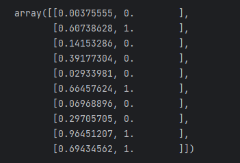

Look, the match is correct. Our task is completed.

The entire process can be demonstrated with the following figure:

Performance Comparison

After the code implementation, we need to compare the Numexpr implementation version with the previous for each implementation version to confirm that there has been a performance improvement.

First, we implement a numexpr_example method. This method is based on the implementation of Numexpr:

def numexpr_example(rows: int) -> np.ndarray:
    orig_arr = generate_ndarray(rows)
    the_result = numexpr_to_binary(orig_arr)
    return the_result

Then, we need to supplement a for_loop_example method. This method refers to the original code I need to rewrite and is used as a performance benchmark:

def for_loop_example(rows: int) -> np.ndarray:
    the_arr = generate_ndarray(rows)
    for i in range(the_arr.shape[0]):
        if the_arr[i][0] < 0.5:
            the_arr[i][0] = 0
        else:
            the_arr[i][0] = 1
    return the_arr

Then, I wrote a test method time_method. This method will generate data from 10 to 10 to the 9th power rows separately, call the corresponding method, and finally save the time required for different data amounts:

def time_method(method: Callable):
    time_dict = dict()
    for i in range(9):
        begin = time.perf_counter()
        rows = 10 ** i
        method(rows)
        end = time.perf_counter()
        time_dict[i] = end - begin
    return time_dict

We test the numexpr version and the for_loop version separately, and use matplotlib to draw the time required for different amounts of data:

t_m = time_method(for_loop_example)
t_m_2 = time_method(numexpr_example)
plt.plot(t_m.keys(), t_m.values(), c="red", linestyle="solid")
plt.plot(t_m_2.keys(), t_m_2.values(), c="green", linestyle="dashed")
plt.legend(["for loop", "numexpr"])
plt.xlabel("exponent")
plt.ylabel("time")
plt.show()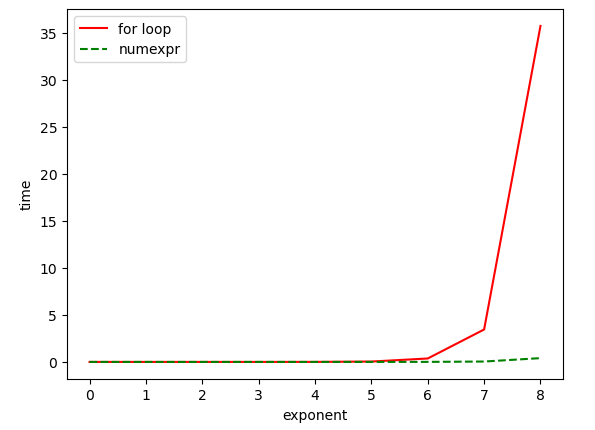

It can be seen that when the number of rows of data is greater than 10 to the 6th power, the Numexpr version of the implementation has a huge performance improvement.

Conclusion

After explaining the basic usage of Numexpr in the previous article, this article uses a specific example in actual work to explain how to use Numexpr to rewrite existing code to obtain performance improvement.

This article mainly uses two features of Numexpr:

1. Numexpr allows calculations to be performed in a vectorized manner.
2. During the calculation of Numexpr, no new arrays will be generated, thereby significantly reducing memory usage.

Thank you for reading. If you have other solutions, please feel free to leave a message and discuss them with me.