Ensuring Correct Use of Transformers in Scikit-learn Pipeline

This article will explain how to use Pipeline and Transformers correctly in Scikit-Learn (sklearn) projects to speed up and reuse our model training process.

This piece complements and clarifies the official documentation on Pipeline examples and some common misunderstandings.

I hope that after reading this, you'll be able to use the Pipeline, an excellent design, to better complete your machine learning tasks.

Introduction

There's a famous dish in Chinese restaurants around the world called "General Tso's Chicken," and I wonder if you've tried it.

One characteristic of "General Tso's Chicken" is that each piece of chicken is processed by the chef to be the same size. This ensures that:

1. All pieces are marinated for the same amount of time.
2. During cooking, each piece of chicken reaches the same level of doneness.
3. When using chopsticks, the uniform size makes it easier to pick up the pieces.

This preprocessing includes washing, cutting, and marinating the ingredients. If the chicken pieces are cut larger than usual, the flavor can change significantly even if stir-fried for the same amount of time.

So, when preparing to open a restaurant, we must consider standardizing these processes and recipes to ensure that each plate of "General Tso's Chicken" has a consistent taste and texture. This is how restaurants thrive.

Back in the world of machine learning, Scikit-Learn also provides such standardized processes called Pipeline. They solidify the data preprocessing and model training process into a standardized workflow, making machine learning projects easier to maintain and reuse.

In this article, we'll explore how to use Transformers correctly within Scikit-Learn's Pipeline, ensuring that our data is as perfectly prepared as the ingredients for a fine meal.

Why Use Transformers

What are Transformers

In Scikit-Learn, Transformers mainly fall into two categories: data scaling and feature dimensionality reduction.

Take, for example, a set of housing data, which includes features like location, area, and number of bedrooms.

If you don't standardize these features to the same scale, the model might overlook the significant impact of location (usually categorical data) due to minor fluctuations in the area (usually a larger numerical value).

It's like overpowering the delicate taste of herbs with too much pepper.

Using Transformers correctly

Typically, data scaling is done using standardization, formulated as:

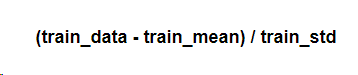
Where train_mean and train_std are variables extracted from the train data.

In Scikit-Learn, train data and test data are both obtained from the original dataset using the train_test_split method.

When scaling test data, the same train_mean and train_std are used:

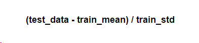
Here arises the question: why use train data to generate these variables?

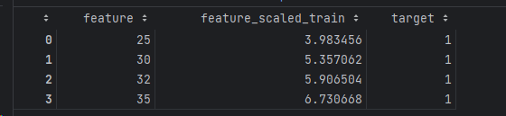
Let's look at a simple dataset where the train data is:

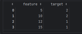
After standardization, the train data becomes:

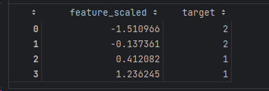
Clearly, after scaling, features greater than 0 have a label of 1, which means features greater than 10 before scaling have a label of 1.

Now let's look at the test data:

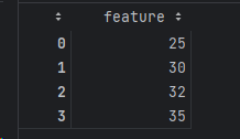
If we use test_mean and test_std generated from the test data distribution without considering the train data, the results become:

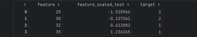
Obviously, this prediction result does not make sense. But suppose we use train_mean and train_std to process the data and combine it with the model prediction; let's see what happens:

As we can see, only by preprocessing the data with variables generated through train data can we ensure that the model's prediction meets expectations.

Using Transformers in Scikit-Learn

Using Transformers in Scikit-Learn is quite simple.

We can generate a set of simulated data using make_classification and then split it into train and test with train_test_split.

from sklearn.datasets import make_classification
from sklearn.model_selection import train_test_split

X, y = make_classification(n_samples=100, n_features=2, 
                           n_classes=2, n_redundant=0, 
                           n_informative=2, n_clusters_per_class=1, 
                           random_state=42)

X_train, X_test, y_train, y_test = train_test_split(X, y, test_size=0.2, random_state=42)

Let's look at the distribution of the data:

import matplotlib.pyplot as plt

plt.scatter(X_train[:, 0], X_train[:, 1], color='red', marker='o')
plt.scatter(X_test[:, 0], X_test[:, 1], color='green', marker='s')
plt.xlabel('feature_idx_0')
plt.ylabel('feature_idx_1')
plt.tight_layout()
plt.show()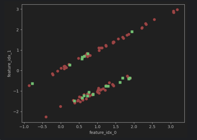

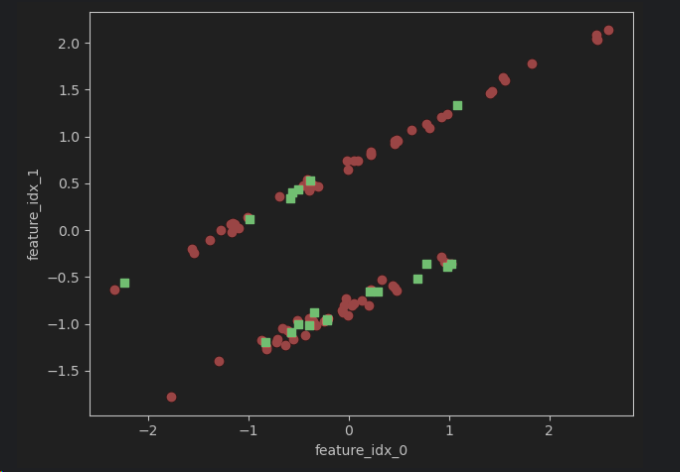
Here we're using StandardScaler to scale the features. First, initialize the StandardScaler, then fit it with train data:

from sklearn.preprocessing import StandardScaler

scaler = StandardScaler()
scaler.fit(X_train)

Next, we can transform the train data's features with the fitted Transformer:

X_train_std = scaler.transform(X_train)

Of course, we could also use fit_transform to fit and transform the train data in one go:

X_train_std = scaler.fit_transform(X_train)

Then we simply transform the test data without needing to fit it again:

X_test_std = scaler.transform(X_test)

After transformation, the distribution of the data remains unchanged, except for the change in scale:

Apart from scaling data with tools like StandardScaler and MinMaxScaler, we can also use PCA, SelectKBest, etc., for dimensionality reduction. For the sake of brevity, I won't delve into these here, but you're welcome to consult the official documentation for more information.

Using Transformers in a Pipeline

Why use a Pipeline

As mentioned earlier, in a machine learning task, we often need to use various Transformers for data scaling and feature dimensionality reduction before training a model.

This presents several challenges:

• Code complexity: For each use of a Transformer, we have to go through initialization, fit_transform, and transform steps. Missing one step during a transformation could derail the entire training process.
• Data leakage: As we discussed, for each Transformer, we fit with train data and then transform both train and test data. We must avoid letting the distribution of the test data leak into the train data.
• Code reusability: A machine learning model includes not only the trained Estimator for prediction but also the data preprocessing steps. Therefore, a machine learning task comprising Transformers and an Estimator should be atomic and indivisible.
• Hyperparameter tuning: After setting up the steps of machine learning, we need to adjust hyperparameters to find the best combination of Transformer parameter values.

Scikit-Learn introduced the Pipeline module to solve these issues.

What is a Pipeline

A Pipeline is a module in Scikit-Learn that implements the chain of responsibility design pattern.

When creating a Pipeline, we use the steps parameter to chain together multiple Transformers for initialization:

from sklearn.pipeline import Pipeline
from sklearn.decomposition import PCA
from sklearn.ensemble import RandomForestClassifier

pipeline = Pipeline(steps=[('scaler', StandardScaler()),
                           ('pca', PCA(n_components=2, random_state=42)),
                           ('estimator', RandomForestClassifier(n_estimators=3, max_depth=5))])

The official documentation points out that the last Transformer must be an Estimator.

If you don't need to specify each Transformer's name, you can simplify the creation of a Pipeline with make_pipeline:

from sklearn.pipeline import make_pipeline

pipeline_2 = make_pipeline(StandardScaler(),
                           PCA(n_components=2, random_state=42),
                           RandomForestClassifier(n_estimators=3, max_depth=5))

Understanding the Pipeline's mechanism from the source code

We've mentioned the importance of not letting test data variables leak into training data when using each Transformer.

This principle is relatively easy to ensure when each data preprocessing step is independent.

But what if we integrate these steps using a Pipeline?

If we look at the official documentation, we find it simply uses the fit method on the entire dataset without explaining how to handle train and test data separately.

With this question in mind, I dived into the Pipeline's source code to find the answer.

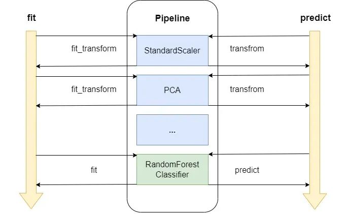
Reading the source code revealed that although Pipeline implements fit, fit_transform, and predict methods, they work differently from regular Transformers.

Take the following Pipeline creation process as an example:

from sklearn.pipeline import Pipeline
from sklearn.decomposition import PCA
from sklearn.ensemble import RandomForestClassifier

pipeline = Pipeline(steps=[('scaler', StandardScaler()),
                           ('pca', PCA(n_components=2, random_state=42)),
                           ('estimator', RandomForestClassifier(n_estimators=3, max_depth=5))])

The internal implementation can be represented by the following diagram:

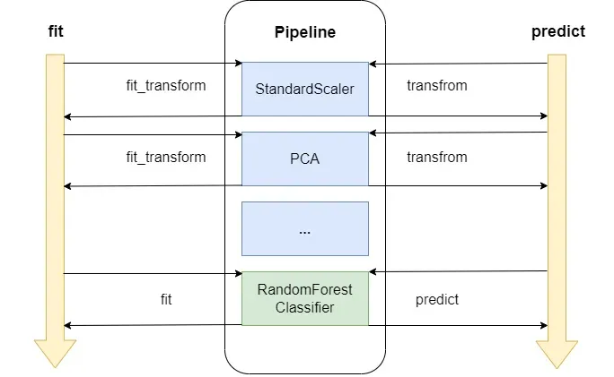
As you can see, when we call the fit method, Pipeline first separates Transformers from the Estimator.

For each Transformer, Pipeline checks if there's a fit_transform method; if so, it calls it; otherwise, it calls fit.

For the Estimator, it calls fit directly.

For the predict method, Pipeline separates Transformers from the Estimator.

Pipeline calls each Transformer's transform method in sequence, followed by the Estimator's predict method.

Therefore, when using a Pipeline, we still need to split train and test data. Then we simply call fit on the train data and predict on the test data.

There's a special case when combining Pipeline with GridSearchCV for hyperparameter tuning: you don't need to manually split train and test data. I'll explain this in more detail in the best practices section.

Best Practices for Using Transformers and Pipeline in Actual Applications

Now that we've discussed the working principles of Transformers and Pipeline, it's time to fulfill the promise made in the title and talk about the best practices when combining Transformers with Pipeline in real projects.

Combining Pipeline with GridSearchCV for hyperparameter tuning

In a machine learning project, selecting the right dataset processing and algorithm is one aspect. After debugging the initial steps, it's time for parameter optimization.

Using GridSearchCV or RandomizedSearchCV, you can try different parameters for the Estimator to find the best fit:

import time

from sklearn.model_selection import GridSearchCV

pipeline = Pipeline(steps=[('scaler', StandardScaler()),
                           ('pca', PCA()),
                           ('estimator', RandomForestClassifier())])
param_grid = {'pca__n_components': [2, 'mle'],
              'estimator__n_estimators': [3, 5, 7],
              'estimator__max_depth': [3, 5]}

start = time.perf_counter()
clf = GridSearchCV(pipeline, param_grid=param_grid, cv=5, n_jobs=4)
clf.fit(X, y)

# It takes 2.39 seconds to finish the search on my laptop.
print(f"It takes {time.perf_counter() - start} seconds to finish the search.")

But in machine learning, hyperparameter tuning is not limited to Estimator parameters; it also involves combinations of Transformer parameters.

Integrating all steps with Pipeline allows for hyperparameter tuning of every element with different parameter combinations.

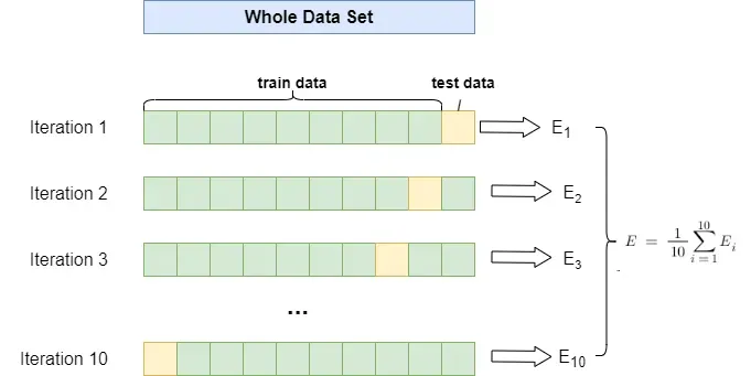
Note that during hyperparameter tuning, we no longer need to manually split train and test data. GridSearchCV will split the data into training and validation sets using StratifiedKFold, which implemented a k-fold cross validation mechanism.

We can also set the number of folds for cross-validation and choose how many workers to use. The tuning process is illustrated in the following diagram:

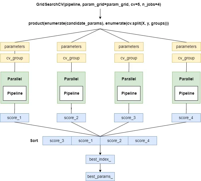
Due to space constraints, I won't go into detail about GridSearchCV and RandomizedSearchCV here. If you're interested, I can write another article explaining them next time.

Using the memory parameter to cache Transformer outputs

Of course, hyperparameter tuning with GridSearchCV can be slow, but that's no worry, Pipeline provides a caching mechanism to speed up the tuning efficiency by caching the results of intermediate steps.

When initializing a Pipeline, you can pass in a memory parameter, which will cache the results after the first call to fit and transform for each transformer.

If subsequent calls to fit and transform use the same parameters, which is very likely during hyperparameter tuning, these steps will directly read the results from the cache instead of recalculating, significantly speeding up the efficiency when running the same Transformer repeatedly.

The memory parameter can accept the following values:

• The default is None: caching is not used.
• A string: providing a path to store the cached results.
• A joblib.Memory object: allows for finer-grained control, such as configuring the storage backend for the cache.

Next, let's use the previous GridSearchCV example, this time adding memory to the Pipeline to see how much speed can be improved:

pipeline_m = Pipeline(steps=[('scaler', StandardScaler()),
                           ('pca', PCA()),
                           ('estimator', RandomForestClassifier())],
                      memory='./cache')
start = time.perf_counter()
clf_m = GridSearchCV(pipeline_m, param_grid=param_grid, cv=5, n_jobs=4)
clf_m.fit(X, y)

# It takes 0.22 seconds to finish the search with memory parameter.
print(f"It takes {time.perf_counter() - start} seconds to finish the search with memory.")

As shown, with caching, the tuning process only takes 0.2 seconds, a significant speed increase from the previous 2.4 seconds.

How to debug Scikit-Learn Pipeline

After integrating Transformers into a Pipeline, the entire preprocessing and transformation process becomes a black box. It can be difficult to understand which step the process is currently on.

Fortunately, we can solve this problem by adding logging to the Pipeline.
We need to create custom transformers to add logging at each step of data transformation.

Here's an example of adding logging with Python's standard logging library:

First, you need to configure a logger:

import logging

from sklearn.base import BaseEstimator, TransformerMixin

logging.basicConfig(level=logging.INFO, format='%(asctime)s - %(levelname)s - %(message)s')
logger = logging.getLogger()

Next, you can create a custom Transformer and add logging within its methods:

class LoggingTransformer(BaseEstimator, TransformerMixin):
    def __init__(self, transformer):
        self.transformer = transformer
        self.real_name = self.transformer.__class__.__name__

    def fit(self, X, y=None):
        logging.info(f"Begin fit: {self.real_name}")
        self.transformer.fit(X, y)
        logging.info(f"End fit: {self.real_name}")
        return self

    def fit_transform(self, X, y=None):
        logging.info(f"Begin fit_transform: {self.real_name}")
        X_fit_transformed = self.transformer.fit_transform(X, y)
        logging.info(f"End fit_transform: {self.real_name}")
        return X_fit_transformed

    def transform(self, X):
        logging.info(f"Begin transform: {self.real_name}")
        X_transformed = self.transformer.transform(X)
        logging.info(f"End transform: {self.real_name}")
        return X_transformed

Then you can use this LoggingTransformer when creating your Pipeline:

pipeline_logging = Pipeline(steps=[('scaler', LoggingTransformer(StandardScaler())),
                             ('pca', LoggingTransformer(PCA(n_components=2))),
                             ('estimator', RandomForestClassifier(n_estimators=5, max_depth=3))])
pipeline_logging.fit(X_train, y_train)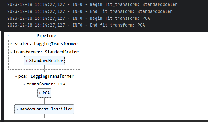

When you use pipeline.fit, it will call the fit and transform methods for each step in turn and log the appropriate messages.

Use passthrough in Scikit-Learn Pipeline

In a Pipeline, a step can be set to 'passthrough', which means that for this specific step, the input data will pass through unchanged to the next step.

This is useful when you want to selectively enable/disable certain steps in a complex pipeline.

Taking the code example above, we know that when using DecisionTree or RandomForest, standardizing the data is unnecessary, so we can use passthrough to skip this step.

An example would be as follows:

param_grid = {'scaler': ['passthrough'],
              'pca__n_components': [2, 'mle'],
              'estimator__n_estimators': [3, 5, 7],
              'estimator__max_depth': [3, 5]}
clf = GridSearchCV(pipeline, param_grid=param_grid, cv=5, n_jobs=4)
clf.fit(X, y)

Reusing the Pipeline

After a journey of trials and tribulations, we finally have a well-performing machine learning model.

Now, you might consider how to reuse this model, share it with colleagues, or deploy it in a production environment.

However, the result of a model's training includes not only the model itself but also the various data processing steps, which all need to be saved.

Using joblib and Pipeline, we can save the entire training process for later use. The following code provides a simple example:

from joblib import dump, load

# save pipeline
dump(pipeline, 'model_pipeline.joblib')

# load pipeline
loaded_pipeline = load('model_pipeline.joblib')

# predict with loaded pipeline
loaded_predictions = loaded_pipeline.predict(X_test)

Conclusion

The official Scikit-Learn documentation is among the best I've seen. By learning its contents, you can master the basics of machine learning applications.

However, when using Scikit-Learn in real projects, we often encounter various details that the official documentation may not cover.

How to correctly combine Transformers with Pipeline is one such case.
In this article, I introduced why to use Transformers and some typical application scenarios.

Then, I interpreted the working principle of Pipeline from the source code level and completed the reasonable use case when applied to train and test datasets.

Finally, for each stage of a real machine learning project, I introduced the best practices of combining Transformers with Pipeline based on my work experience.

I hope this article can help you. If you have any questions, please leave me a message, and I will try my best to answer them.