Exploring Numexpr: A Powerful Engine Behind Pandas

This article will introduce you to the Python library Numexpr, a tool that boosts the computational performance of Numpy Arrays. The eval and query methods of Pandas are also based on this library.

This article also includes a hands-on weather data analysis project.

By reading this article, you will understand the principles of Numexpr and how to use this powerful tool to speed up your calculations in reality.

Introduction

Recalling Numpy Arrays

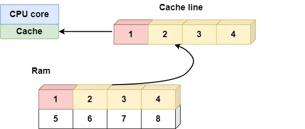
In a previous article discussing Numpy Arrays, I used a library example to explain why Numpy's Cache Locality is so efficient:

Python Lists Vs. NumPy Arrays: A Deep Dive into Memory Layout and Performance Benefits

Exploring allocation differences and efficiency gains

Data Leads FuturePeng Qian

Each time you go to the library to search for materials, you take out a few books related to the content and place them next to your desk.

This way, you can quickly check related materials without having to run to the shelf each time you need to read a book.

This method saves a lot of time, especially when you need to consult many related books.

In this scenario, the shelf is like your memory, the desk is equivalent to the CPU's L1 cache, and you, the reader, are the CPU's core.

The limitations of Numpy

Suppose you are unfortunate enough to encounter a demanding professor who wants you to take out Shakespeare and Tolstoy's works for a cross-comparison.

At this point, taking out related books in advance will not work well.

First, your desk space is limited and cannot hold all the books of these two masters at the same time, not to mention the reading notes that will be generated during the comparison process.

Second, you're just one person, and comparing so many works would take too long. It would be nice if you could find a few more people to help.

This is the current situation when we use Numpy to deal with large amounts of data:

• The number of elements in the Array is too large to fit into the CPU's L1 cache.
• Numpy's element-level operations are single-threaded and cannot utilize the computing power of multi-core CPUs.

What should we do?

Don't worry. When you really encounter a problem with too much data, you can call on our protagonist today, Numexpr, to help.

Understanding Numexpr: What and Why

How it works

When Numpy encounters large arrays, element-wise calculations will experience two extremes.

Let me give you an example to illustrate. Suppose there are two large Numpy ndarrays:

import numpy as np
import numexpr as ne

a = np.random.rand(100_000_000)
b = np.random.rand(100_000_000)

When calculating the result of the expression a**5 + 2 * b, there are generally two methods:

One way is Numpy's vectorized calculation method, which uses two temporary arrays to store the results of a**5 and 2*b separately.

In: %timeit a**5 + 2 * b

Out:2.11 s ± 31.1 ms per loop (mean ± std. dev. of 7 runs, 1 loop each)

At this time, you have four arrays in your memory: a, b, a**5, and 2 * b. This method will cause a lot of memory waste.

Moreover, since each Array's size exceeds the CPU cache's capacity, it cannot use it well.

Another way is to traverse each element in two arrays and calculate them separately.

c = np.empty(100_000_000, dtype=np.uint32)

def calcu_elements(a, b, c):
    for i in range(0, len(a), 1):
        c[i] = a[i] ** 5 + 2 * b[i]
        
%timeit calcu_elements(a, b, c)


Out: 24.6 s ± 48.2 ms per loop (mean ± std. dev. of 7 runs, 1 loop each)

This method performs even worse. The calculation will be very slow because it cannot use vectorized calculations and only partially utilize the CPU cache.

Numexpr's calculation

Numexpr commonly uses only one evaluate method. This method will receive an expression string each time and then compile it into bytecode using Python's compile method.

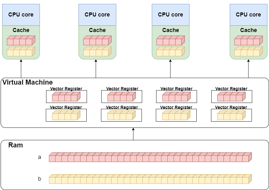
Numexpr also has a virtual machine program. The virtual machine contains multiple vector registers, each using a chunk size of 4096.

When Numexpr starts to calculate, it sends the data in one or more registers to the CPU's L1 cache each time. This way, there won't be a situation where the memory is too slow, and the CPU waits for data.

At the same time, Numexpr's virtual machine is written in C, removing Python's GIL. It can utilize the computing power of multi-core CPUs.

So, Numexpr is faster when calculating large arrays than using Numpy alone. We can make a comparison:

In:  %timeit ne.evaluate('a**5 + 2 * b')
Out: 258 ms ± 14.4 ms per loop (mean ± std. dev. of 7 runs, 1 loop each)

Summary of Numexpr's working principle

Let's summarize the working principle of Numexpr and see why Numexpr is so fast:

Executing bytecode through a virtual machine. Numexpr uses bytecode to execute expressions, which can fully utilize the branch prediction ability of the CPU, which is faster than using Python expressions.

Vectorized calculation. Numexpr will use SIMD (Single Instruction, Multiple Data) technology to improve computing efficiency significantly for the same operation on the data in each register.

Multi-core parallel computing. Numexpr's virtual machine can decompose each task into multiple subtasks. They are executed in parallel on multiple CPU cores.

Less memory usage. Unlike Numpy, which needs to generate intermediate arrays, Numexpr only loads a small amount of data when necessary, significantly reducing memory usage.

Numexpr and Pandas: A Powerful Combination

You might be wondering: We usually do data analysis with pandas. I understand the performance improvements Numexpr offers for Numpy, but does it have the same improvement for Pandas?

The answer is Yes.

The eval and query methods in pandas are implemented based on Numexpr. Let's look at some examples:

Pandas.eval for Cross-DataFrame operations

When you have multiple pandas DataFrames, you can use pandas.eval to perform operations between DataFrame objects, for example:

import pandas as pd

nrows, ncols = 1_000_000, 100
df1, df2, df3, df4 = (pd.DataFrame(rng.random((nrows, ncols))) for i in range(4))

If you calculate the sum of these DataFrames using the traditional pandas method, the time consumed is:

In:  %timeit df1+df2+df3+df4
Out: 1.18 s ± 65.1 ms per loop (mean ± std. dev. of 7 runs, 1 loop each)

You can also use pandas.eval for calculation. The time consumed is:

In:  %timeit pd.eval('df1 + df2 + df3 + df4')
Out: 452 ms ± 29.4 ms per loop (mean ± std. dev. of 7 runs, 1 loop each)

The calculation of the eval version can improve performance by 50%, and the results are precisely the same:

In:  np.allclose(df1+df2+df3+df4, pd.eval('df1+df2+df3+df4'))
Out: True

DataFrame.eval for column-level operations

Just like pandas.eval, DataFrame also has its own eval method. We can use this method for column-level operations within DataFrame, for example:

df = pd.DataFrame(rng.random((1000, 3)), columns=['A', 'B', 'C'])

result1 = (df['A'] + df['B']) / (df['C'] - 1)
result2 = df.eval('(A + B) / (C - 1)')

The results of using the traditional pandas method and the eval method are precisely the same:

In:  np.allclose(result1, result2)
Out: True

Of course, you can also directly use the eval expression to add new columns to the DataFrame, which is very convenient:

df.eval('D = (A + B) / C', inplace=True)
df.head()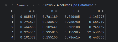

Using DataFrame.query to quickly find data

If the eval method of DataFrame executes comparison expressions, the returned result is a boolean result that meets the conditions. You need to use Mask Indexing to get the desired data:

mask = df.eval('(A < 0.5) & (B < 0.5)')
result1 = df[mask]
result1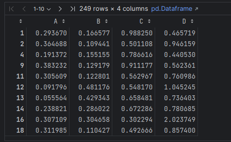

The DataFrame.query method encapsulates this process, and you can directly obtain the desired data with the query method:

In:   result2 = df.query('A < 0.5 and B < 0.5')
      np.allclose(result1, result2)
Out:  True

When you need to use scalars in expressions, you can use the @ symbol to indicate:

In:  Cmean = df['C'].mean()
     result1 = df[(df.A < Cmean) & (df.B < Cmean)]
     result2 = df.query('A < @Cmean and B < @Cmean')
     np.allclose(result1, result2)
Out: True

Practical Example: Using Numexpr and Pandas in Real-World Scenarios

In all articles explaining Numexpr, examples are made using synthetic data. This feeling is not good and may cause you to not know how to use this powerful library to complete tasks after reading the article.

Therefore, in this article, I will take a weather data analysis project as an example to explain how we should use Numexpr to process large datasets in actual work.

Project Goal

After a hot summer, I really want to see if there is such a place where the climate is pleasant in summer and suitable for me to escape the heat.

This place should meet the following conditions:

1. In the summer:
2. The daily average temperature is between 18 degrees Celsius and 22 degrees Celsius;
3. The diurnal temperature difference is between 4 degrees Celsius and 6 degrees Celsius;
4. The average wind speed in kmh is between 6 and 10. It would feel nice to have a breeze blowing on me.

Data preparation

This time, I used the global major city weather data provided by the Meteostat JSON API.

The data is licensed under the Creative Commons Attribution-NonCommercial 4.0 International Public License (CC BY-NC 4.0) and can be used commercially.

I used the parquet dataset integrated on Kaggle based on the Meteostat JSON API for convenience.

I used version 2.0 of pandas. The pandas.read_parquet method of this version can easily read parquet data. But before reading, you need to install Pyarrow and Fastparquet.

conda install pyarrow

conda install fastparquet

Data analysis

After the preliminary preparations, we officially entered the data analysis process.

First, I read the data into memory and then look at the situation of this dataset:

import os
from pathlib import Path

import pandas as pd

root = Path(os.path.abspath("")).parents[0]
data = root/"data"

df = pd.read_parquet(data/"daily_weather.parquet")
df.info()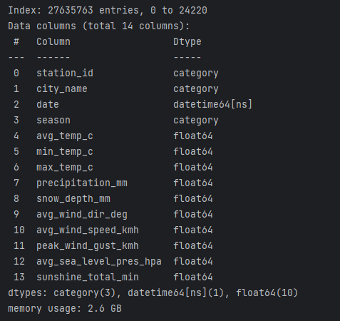

As shown in the figure, this dataset contains 13 fields. According to the goal of this project, I plan to use the fields of city_name, season, min_temp_c, max_temp_c, avg_wind_speed_kmh.

Next, I first remove the data in the corresponding fields that contain empty values for subsequent calculations, and then select the desired fields to form a new DataFrame:

sea_level_not_null = df.dropna(subset=['min_temp_c', 'max_temp_c', 'avg_wind_speed_kmh'] , how='any')

sample = sea_level_not_null[['city_name', 'season',
                             'min_temp_c', 'max_temp_c', 'avg_wind_speed_kmh']]

Since I need to calculate the average temperature and temperature difference, I use the Pandas.eval method to directly calculate the new indicators on the DataFrame:

sample.eval('avg_temp_c = (max_temp_c + min_temp_c) / 2', inplace=True)
sample.eval('diff_in_temp = max_temp_c - min_temp_c', inplace=True)

Then, average a few indicators by city_name and season:

sample = sample.groupby(['city_name', 'season'])\
        [['min_temp_c', 'max_temp_c', 'avg_temp_c', 'diff_in_temp', 'avg_wind_speed_kmh']]\
            .mean().round(1).reset_index()
            
sample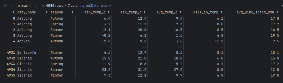

Finally, according to the goal of the project, I use DataFrame.query to filter the dataset:

sample.query('season=="Summer" \
        & 18 < avg_temp_c < 22 \
        & 4 < diff_in_temp < 6 \
        & 6 < avg_wind_speed_kmh < 10')

The final result is out. Only one city meets my requirements: Vladivostok, a non-freezing port in the east of Russia. It is indeed an excellent place to escape the heat!

Best Practices and Takeaways

After explaining the project practice of Numexpr, as usual, I will explain some of the best practices of Numexpr combined with my own work experience for you.

Avoid overuse

Although Numexpr and pandas eval have significant performance advantages when handling large data sets. However, dealing with small data sets is not faster than regular operations.

Therefore, you should choose whether to use Numexpr based on the size and complexity of the data. And my experience is to use it when you feel the need, as small datasets won't slow things down too much anyway.

The use of the eval function is limited

The eval function does not support all Python and pandas operations.

Therefore, before using it, you should consult the documentation to understand what operations eval supports.

Be careful when handling strings

Although I used season="Summer" to filter the dataset in the project practice, the eval function is not very fast when dealing with strings.

If you have a lot of string operations in your project, you need to consider other ways.

Be mindful of memory usage

Although Numexpr no longer generates intermediate arrays, large datasets will occupy a lot of memory.

For example, the dataset occupies 2.6G of memory in my project example. At this time, you have to be very careful to avoid the program crashing due to insufficient memory.

Use the appropriate data type

This point is detailed in the official documentation, so I won't repeat it here.

Use the inplace parameter when needed

Using the inplace parameter of the DataFrame.eval method can directly modify the original dataset, avoiding generating a new dataset and occupying a lot of memory.

Of course, doing so will lead to modifications to the original dataset, so please be careful.

Conclusion

In this article, I brought a comprehensive tutorial on Numexpr, including:

The applicable scenarios of Numexpr, the effect of performance improvement, and its working principle.

The eval and query methods in Pandas are also based on Numexpr. It will bring great convenience and performance improvement to your pandas' operations if used appropriately.

Through a global weather data analysis project, I demonstrated how to use pandas' eval and query methods in practice.

As always, combined with my work experience, I introduced the best practices of Numexpar and the eval method of pandas.

Thank you for reading. If you have any questions, please leave a message in the comment area, and I will answer in time.