Efficient k-Nearest Neighbors (k-NN) Solutions with NumPy

Introduction

I have a friend who is a city planner. One day, he was tasked with reassessing the location suitability of thousands of gas stations in the city, needing to find the positions of the k-nearest gas stations to each one.

How can we find the nearest k stations with little time? This is a practical application scenario of the k-nearest neighbors problem.

As such, he came to me for help, hoping I could provide a high-performance solution.

So I write down this article and which will guide you on efficiently solving the k-nearest neighbors problem using NumPy. By comparing it with a Python iterative solution, we will demonstrate the powerful performance of NumPy.

In this article, we will delve into utilizing advanced NumPy features, such as broadcasting, fancy indexing, and sorting, to implement a high-performance k-nearest neighbors algorithm.

After reading this article, you will able to:

• Understand the k-nearest neighbors problem and its practical application scenarios
• Learn how to use the NumPy library to solve the k-nearest neighbors problem
• Understand in-depth how features such as NumPy broadcasting, fancy indexing, and sorting play a role in the algorithm
• Compare the performance of NumPy with a Python iterative solution, exploring why NumPy is superior

Let’s delve into the high-performance world of NumPy together, exploring how we can solve the k-nearest neighbors problem more quickly and effectively using only NumPy.

Geometric Principles of Solving the k-NN Problem

Let’s review the gas station problem my friend faced from a geometric perspective.

Assuming we place all the gas stations on a two-dimensional plane, the distance between two gas stations is actually the Euclidean distance between two points on the plane. The solution formula is as follows:

But how should the distance between any two points be calculated?

We can imagine the two-dimensional plane as a chessboard, simplify the gas stations to six, and sequentially arrange these six points along the horizontal and vertical edges of the chessboard, as shown in the figure:

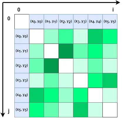
Then the grid where the extensions of any two points intersect can represent the distance between these two points. When i=j, the two points are the same, and the distance should be 0.

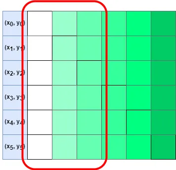
Assuming that k=2 here, we only need to sort the distances from each point to other points in ascending order and take the points corresponding to the first three distances (including itself), which are the two closest other points to this point.

Traditional Python Iterative Solution

As a performance benchmark, let’s first look at how the traditional Python iterative solution works.

The idea of this solution is relatively simple:

1. To calculate the Euclidean distance between the coordinate point itself and other coordinate points in the list.
2. Then compare the distances from the current point to other points.
3. Take the top k points that meet the requirements.

Next is the code part.

First, we randomly generate six coordinate points. Since we will use the same coordinates as a comparison later, we need to add a seed to the random package.

import random
import matplotlib.pyplot as plt

%matplotlib inline
plt.style.use('seaborn-v0_8-whitegrid')
random.seed(5)


def generate_points(n: int=6) -> list[tuple]:
    points = []
    for i in range(n):
        points.append((random.randint(0, 100), random.randint(0, 100)))
    return points

Next, start calculating the distance of each point to all points (including itself) in the list, which requires two iterations.

def calc_dist(points: list[tuple]) -> list[list]:
    result = []
    for i, left in enumerate(points):
        row = [left]
        for j, right in enumerate(points):
            dist = (left[0] - right[0])**2 + (left[1] - right[1])**2
            row.append(dist)
        result.append(row)
    return result

Then, sort the distances between each point and other points and find the index of the point corresponding to the distance in the original list.

def find_sorted_index(with_dist: list[list]) -> list[list]:
    results = []
    for row in with_dist:
        dists = row[1:]
        sorted_dists = sorted(dists)
        indices = [dists.index(i) for i in sorted_dists]
        row[1:] = indices
        results.append(row)
    return results

The final return should be a two-dimensional array, where the first item in each row of the array is the current point, and the other items are the indexes of each point in the list after sorting the distance.

Finally, we find each point that meets the conditions in the original coordinate list based on the index.

def find_k_nearest(points: list[tuple], with_indices: list[list], k: int) -> list[tuple]:
    results = []
    for row in with_indices:
        # Since the closest point to the current point is itself, we can get the point itself directly, so here is +2
        k_indices = row[1:k+2]
        the_points = [points[i] for i in k_indices]
        results.append(the_points)
    return results

The result is a two-dimensional array, and each row of the array is the current point and the other two closest points.

To facilitate our evaluation of the results, we use Matplotlib to draw all coordinate points and the lines from each coordinate to the two nearest coordinates.

def draw_points(points: list[tuple]):
    x, y = [], []
    for point in points:
        x.append(point[0])
        y.append(point[1])
    plt.scatter(x, y, s=100)


def draw_lines(nearest: list[list]):
    for row in nearest:
        start = row[0]
        for end in row[1:]:
            plt.plot([start[0], end[0]], [start[1], end[1]], color='black')


def orig_main(count: int = 6):
    k = 2
    points = generate_points(count)
    with_dist = calc_dist(points)
    sorted_index = find_sorted_index(with_dist)
    nearest = find_k_nearest(points, sorted_index, k)
    return points, nearest


points, nearest =  orig_main(6)
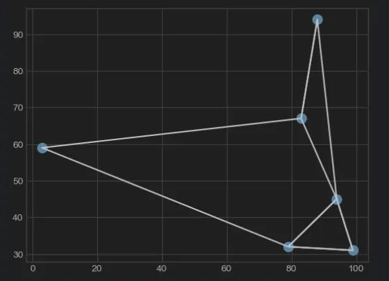
draw_points(points)
draw_lines(nearest)

The result is as follows:

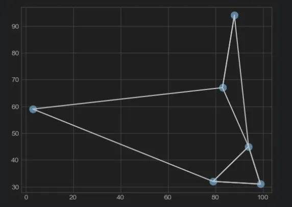
As you can see, six coordinates and corresponding lines have appeared on the chart.

This chart will serve as a benchmark and will be compared with the results of using NumPy later to confirm the correctness of the algorithm.

Basic Knowledge of Using NumPy Solution

Next, let’s see how to solve this problem using NumPy.

Before writing the code, we need to do some preheating on some basic concepts of NumPy.

Broadcasting

Since it involves placing a set of coordinate points on the chessboard horizontally (shape=(1, 6)) and vertically (shape=(6, 1)), and forming a (6, 6) matrix.

After calculating the distance, it involves operations between two arrays of different sizes, so we need to use the broadcasting mechanism of NumPy.

Here is an example:

In:    a = np.arange(6).reshape(1, 6)
       b = np.arange(6).reshape(6, 1)
       a + b
Out:   [[ 0  1  2  3  4  5]
        [ 1  2  3  4  5  6]
        [ 2  3  4  5  6  7]
        [ 3  4  5  6  7  8]
        [ 4  5  6  7  8  9]
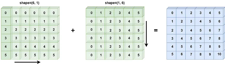
        [ 5  6  7  8  9 10]]

As you can see, when a (1, 6) array and a (6, 1) array are added, the resulting shape is (6, 6).

For the specific principles, please refer to the official documentation. The schematic diagram is as follows:

Sorting

After solving the distance between any two points, we also need to sort the distances.

Like the sort() function in the Python standard library, NumPy also has a function for sorting: np.sort(). Alternatively, the ndarray.sort() function can also be used for sorting.

Since we are sorting the distances, we also need to find the index of each item in the original array after sorting. In NumPy, we can use np.argsort() to get it:

In:  x = np.array([2, 1, 4, 3, 5])
     i = np.argsort(x)
     print(i)
Out: [1 0 3 2 4]

Of course, we only need to focus on the k-nearest points, and we don’t need to know the order of distances.

So we can use NumPy’s argpartition() API, which can return the index of the smallest few points without sorting, which will perform better.

Fancy Indexing

In the traditional Python list, if we want to find a set of data by index, we need to iterate separately through the data list and index list, which has very poor performance.

But NumPy provides fancy indexing to quickly find data corresponding to the index. Here is an example:

In:  x = np.array([8, 2, 4, 5, 3, 7, 1, 6])
     ind = [0, 3, 7]
     print(x[ind])
Out: [8 5 6]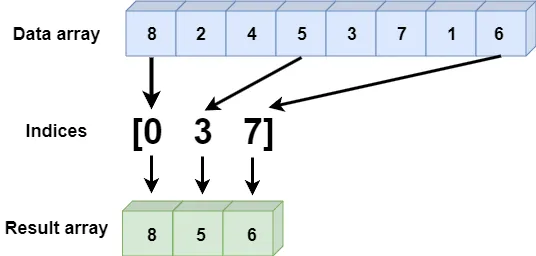

Because fancy indexing is a set of integer arrays, there is a rule to follow:

The data indexed reflects the shape of the broadcasted index array, which is unrelated to the shape of the data array.

NumPy Solution

After understanding some basics of NumPy, let’s see how to solve the k-NN problem using NumPy.

Since here we are using a set of coordinate points to form an array, we need to use NumPy’s structured_array:

import numpy as np
from numpy import ndarray

random.seed(5)

def structured_array(points: list[tuple]) -> ndarray:
    dt = np.dtype([('x', 'int'), ('y', 'int')])
    return np.array(points, dtype=dt)

Next, add an extra dimension to the original one-dimensional array in the horizontal and vertical directions, turning it into two sides of a two-dimensional chessboard:

Then use the broadcasting mechanism to calculate the distance between each point.

Finally, get a (6, 6) two-dimensional array:

def np_find_dist(s_array: ndarray) -> ndarray:
    a = s_array.reshape(6, 1)
    b = s_array.reshape(1, 6)
    dist = (a['x'] - b['x'])**2 + (a['y'] - b['y'])**2
    return dist

Then, use the argpartition method to find out the indexes of the two points with the smallest distance in each row:

def np_k_nearest(dist: ndarray, k: int) -> ndarray:
    k_indices = np.argpartition(dist, k+1, axis=1)[:, :k+1]
    return k_indices

We still need two Matplotlib drawing methods to evaluate the correctness of the results:

def np_draw_points(s_array: ndarray):
    plt.scatter(s_array['x'], s_array['y'], s=100)


def np_draw_lines(s_array: ndarray, k_indices: ndarray, k: int):
    for i in range(s_array.shape[0]):
        for j in k_indices[i, :k+1]:
            plt.plot([s_array[i]['x'], s_array[j]['x']],
                     [s_array[i]['y'], s_array[j]['y']],
                     color='black')

Finally, write a main method to integrate all the code together:

def np_main(count: int = 6):
    k = 2
    points = generate_points(count)
    s_array = structured_array(points)
    np_dist = np_find_dist(s_array)
    k_indices = np_k_nearest(np_dist, k)

    results = [s_array[k_indices[i, :k+1]] 
               for i in range(s_array.shape[0])]
    return results, s_array, k_indices, k


results, s_array, k_indices, k = np_main(6)
np_draw_points(s_array)
np_draw_lines(s_array, k_indices, k)

Just looking at the code, it’s already much simpler than the Python iterative version. Next, we compare the results with the chart:

See, the results are exactly the same!

Performance Comparison of the Two Solutions

Finally, let’s compare the execution performance of the two solutions. Here we still use %timeit for evaluation.

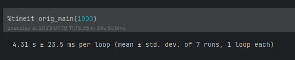
First is the Python iterative way. Let’s see how long it takes to expand to 1,000 coordinates:

Then it’s the NumPy implementation. See how long it takes for 1,000 coordinates:

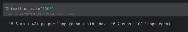
Surprised, right? The performance has improved hundreds of times, so my friend doesn’t have to worry about being unable to calculate it.

Conclusion

This article taught us how to use NumPy’s broadcasting, fancy indexing, and sorting to efficiently solve the k-nearest neighbors problem.

We also compared the performance of NumPy with the Python iterative solution and deeply understood why NumPy can perform better in solving such problems.

To recap, we learned the following:

• The definition and practical application scenarios of the k-nearest neighbors problem
• How to use the NumPy library to solve the k-nearest neighbors problem
• The application of NumPy’s broadcasting, fancy indexing, sorting, and other features in algorithm implementation
• The performance comparison analysis between NumPy and the Python brute force solution

Although this article provides an efficient k-nearest neighbors solution, this is just a starting point.

In future articles, I will reinterpret the solution to this problem using advanced algorithms and data structures, showing you more efficient and usable algorithm skills.

Stay tuned for future articles. If you are interested in this article, feel free to comment, and I will answer them individually.